Manufacturing planning with pickup and delivery
This guide describes manufacturing planning in JOpt.TourOptimizer: with the FlexLoads of the pickup and delivery (PND) module, the optimizer decides how much a production site produces, which site produces it and when the goods need to be ready. Production quantities are not set by the user but optimized together with routing, scheduling and capacity constraints. The guide is written for developers who model supply and demand with the PND module; the pickup and delivery guide explains the load types and depots it builds on.
Table of contents
What it does
The key mechanism is the SupplyFlexLoad. With a SimpleLoad, the user defines a fixed quantity. With a SupplyFlexLoad, the optimizer determines the supply quantity at a node:
- A node is modeled as a production site (factory, bakery, warehouse).
- The node carries a
SupplyFlexLoadwith a load type, for example "Bread", but no fixed quantity. - The optimizer decides how many units this node produces, based on routing, capacity, time windows and demand across the whole problem.
- The production quantity appears in the optimization result next to the route schedule.
The user defines what can be produced and where. The optimizer decides how much and distributes it across the network.
FlexLoad types
Manufacturing planning is one application of the FlexLoad family. JOpt provides FlexLoad types for different scenarios:
| FlexLoad type | What the optimizer decides | Typical use case |
|---|---|---|
SupplyFlexLoad | How much a node produces | Factory output planning, bakery production |
RequestFlexLoad | How much a node requests | Flexible demand, partial fulfillment |
MixedFlexLoad | Whether a node supplies or requests, and how much | Warehouse buffers, reload and unload points |
TimedSupplyFlexLoad | How much a node produces, for requests with a delivery time limit (SLA) | Pizza delivery chains, time-critical production |
These types can be combined in one optimization. A scenario can hold fixed deliveries (SimpleLoad), flexible production (SupplyFlexLoad), warehouse buffers (MixedFlexLoad) and timed delivery promises (TimedSupplyFlexLoad) in one problem instance.
How the optimizer searches
Dynamic production planning inside a route optimizer is a hard problem. The optimizer must simultaneously decide quantities, assignments, and routes. This works in JOpt because the engine uses a multi-phase pipeline with dedicated operators for PND problems:
- Construction phase. The starting solution allocates demands to resources and estimates initial supply quantities using savings-based heuristics or clustering.
- Simulated annealing. The solution is refined through neighborhood moves that include both route changes and supply adjustments. FlexLoad quantities are modified alongside node ordering.
- Genetic algorithm with dedicated PND operators. The genetic algorithm uses both random operators (mutations and crossings, as in nature) and intelligent operators that evaluate solutions before and after modification. For PND problems, these operators understand goods tracking: they can adjust production quantities, swap supply assignments between facilities, and rebalance loads across routes. This is not a generic constraint solver trying random moves. The operators are specifically designed to explore the production-routing search space efficiently.
- Feasibility tracking. Throughout all phases, JOpt tracks goods in vehicles at every point in the route. Overloading and underloading are detected and penalized through cost, giving the optimizer a strong incentive to find balanced solutions while still allowing it to explore intermediate states that temporarily violate capacity. This cost-based approach is deliberate: it gives the genetic operators the freedom to rearrange production quantities and delivery assignments without being locked out of promising regions of the search space.
Because the genetic algorithm evaluates many solution candidates in parallel and the dedicated operators make intelligent production-aware moves, the optimizer converges to good production plans even in large instances with dozens of facilities and hundreds of delivery points.
Split delivery
CoupledRequestFlexLoad is experimental: you can use it, and its API or behaviour may still change. The coupled split delivery page shows it with an example.The FlexLoad concept extends to split delivery optimization (SDO). In many real-world scenarios, a large order does not have to be delivered in one piece. A supermarket ordering 50 pallets might accept two deliveries of 25 on different days or from different trucks. A construction site receiving building materials might have several unloading bays at different positions on the site. Splitting a delivery can dramatically improve overall route efficiency, vehicle utilization and schedule feasibility.
JOpt supports this through coupled FlexLoads. Several nodes, each with its own NodeDepot and loads, are coupled together. When the optimizer increases the load at one node, the load of the coupled node decreases by the same amount. This way, one demand can be split across several delivery points, each a node of its own with its own location, time window and visit duration.
The user can define the maximum number of splits allowed for a single load. Each split node can be placed at a different geographical position if the delivery scenario requires it. Optionally, the visit duration at each split node can be defined as a function of the delivered quantity, so that a partial delivery of 10 pallets takes less time than a full delivery of 50. This makes the model realistic: smaller deliveries are faster to unload.
The advantage is significant. To our best knowledge, classical VRP solvers treat each delivery as an atomic unit: one customer, one visit, one fixed quantity. If a single large order blocks an entire truck for a full shift, the rest of the route suffers. With split delivery optimization, the optimizer can distribute that order across vehicles, shifts, or partial visits in a way that is globally optimal. It reduces vehicle overload situations, improves capacity utilization across the fleet, and opens scheduling options that are simply invisible to solvers without this capability.
Technically, the mechanism is called CoupledRequestFlexLoad. It builds on the same FlexLoad infrastructure used for manufacturing planning, reusing the dedicated PND operators in the genetic algorithm. The coupling is bidirectional: the optimizer explores different split ratios as part of its search, evaluating many candidate distributions through the same multi-phase pipeline (construction, simulated annealing, genetic search) that handles all other PND decisions.
CoupledRequestFlexLoad can be combined with SupplyFlexLoad nodes, for example in multi-day scenarios. When the optimizer splits a delivery across days, the resource starts empty at its base each morning and needs to load exactly the right quantity before it visits the split delivery node. A SupplyFlexLoad at a warehouse or a production site provides it. For example, a customer requests 30 pallets, and the optimizer splits them into 10 on day one and 20 on day two. On day one, the truck starts empty at the base, loads 10 at the SupplyFlexLoad and serves the CoupledRequestFlexLoad with 10. On day two, it loads 20 and delivers the rest. The optimizer determines the split ratio and the loading quantities as one coordinated decision.
When to use it
Use manufacturing planning when production and delivery are tightly coupled. A bakery does not want to produce bread that nobody ordered. A pizza restaurant chain needs to decide which branch prepares which order.
Traditionally, these decisions are made in two separate steps: first a production planner decides the quantities per facility, then a route optimizer plans the deliveries. With this separation, production decisions are made without knowledge of the routing costs, and routing decisions are made without flexibility on supply. JOpt considers production quantities, facility assignments, routing, time windows and capacity constraints as one problem and plans production and delivery together.
Other routing engines
To our best knowledge, this capability is unique among route optimization engines: other common VRP solvers do not offer a built-in mechanism where the optimizer dynamically determines production quantities as part of the routing solution, and in these engines, supply quantities must be fixed before optimization begins. JOpt does not have this limitation.
We surveyed the most widely used open-source VRP solvers to understand how they handle dynamic supply decisions.
In JOpt, production quantities are planning variables that the optimizer controls. To our best knowledge, in other engines they are input data that must be fixed before optimization starts. This means JOpt can answer questions that, to our best knowledge, other engines cannot even formulate:
- How much should each factory produce?
- Which production site should serve which customer?
- What is the jointly optimal production and delivery plan?
- Should a large order be split across several vehicles or visits, and if so, in what ratio?
These questions belong to production and distribution planning, and JOpt answers them inside the route optimizer. This integration is possible because JOpt has dedicated genetic operators for PND that understand goods creation, goods tracking, load splitting and load balancing as first-class concepts in the search process.
How to use it
The bakery example
A bakery company has two production sites: Bakery Aachen and Bakery Cologne. Each production site has one delivery driver (a resource) and a truck with a maximum capacity of 20 bread trays. Several supermarkets in the region need bread deliveries, each with a defined demand. The values are those of the bakery example.
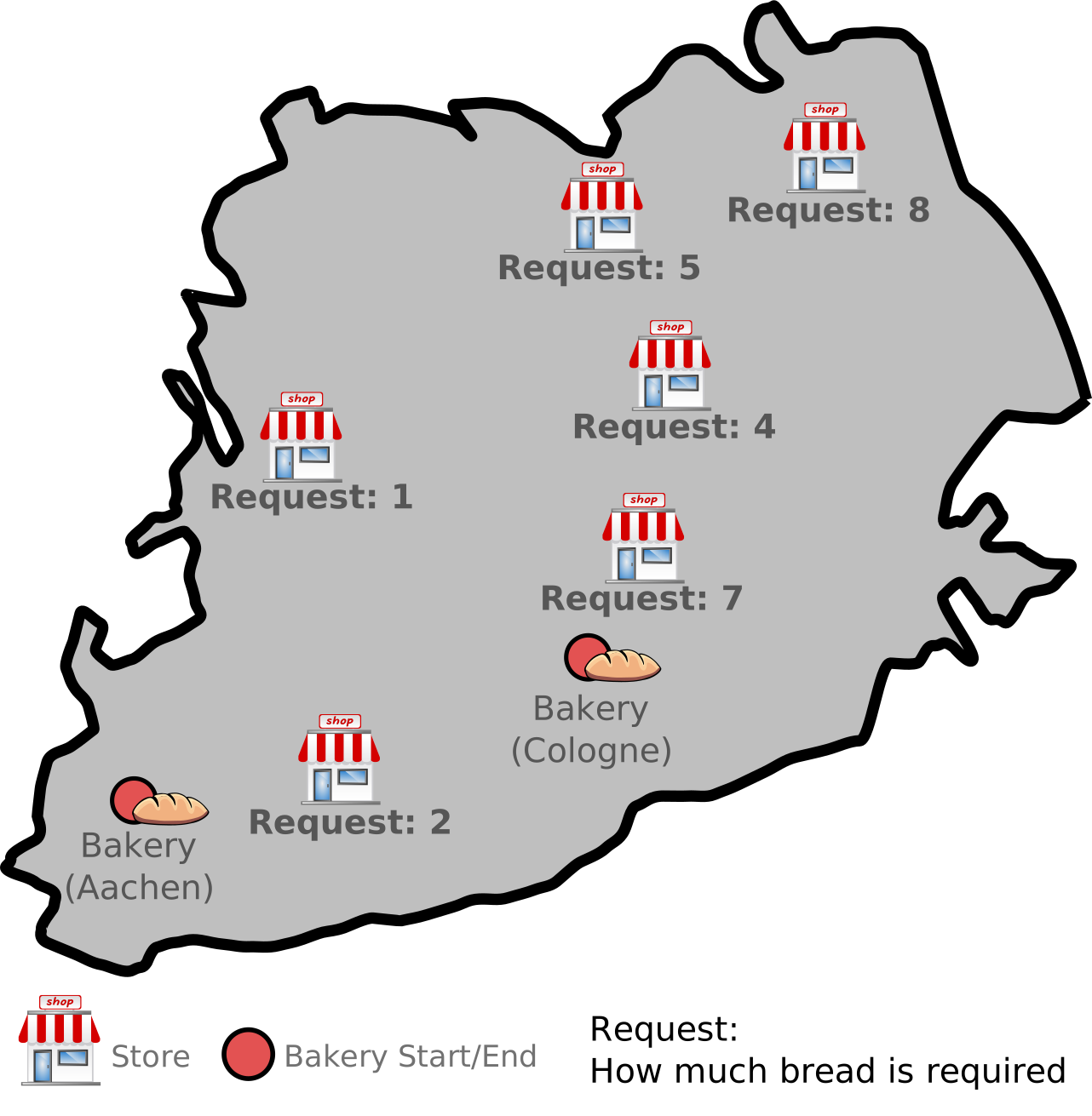
Figure 1: Two bakeries and six stores with their demand. The optimizer decides how much each bakery produces.
The company does not want to overproduce (waste) or underproduce (missed demand). Instead of deciding the production quantities by hand, it adds two SupplyFlexLoad nodes, one near each bakery. These nodes act as factories that can produce bread. The optimizer determines the production quantity of each factory from the total demand, the truck capacity, the route distances and the time windows.
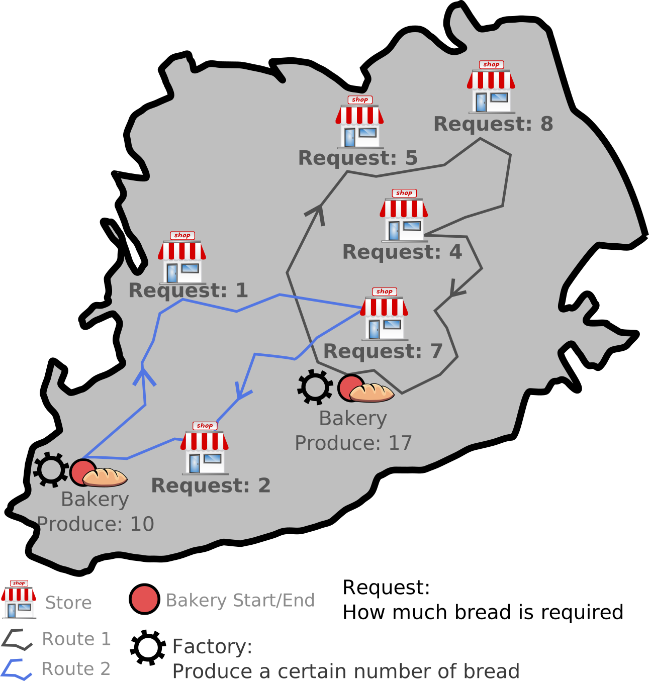
Figure 2: The optimized result. Bakery Aachen produces 10 trays, and Bakery Cologne produces 17 trays.
The result is a complete plan: how much each bakery produces, which truck delivers to which supermarket, and in what order. Production planning and route optimization are solved in one run.
Implementation sketch in Java
A SupplyFlexLoad is created with a load ID and attached to a NodeDepot at the production node:
// Create a supply flex load for bread production
ILoad breadSupply = new SupplyFlexLoad("Bread", 20, true);

// Create a node depot and add the flex load
INodeDepot bakeryDepot = new SimpleNodeDepot("BakeryDepot");
bakeryDepot.add(breadSupply);

// Attach to the bakery node
bakeryNode.setNodeDepot(bakeryDepot);
The second parameter (20) defines the maximum capacity the SupplyFlexLoad can provide. The third parameter (true) enables fuzzy behavior, allowing partial supply. The optimizer determines the actual quantity during the optimization.
On the demand side, the supermarkets carry standard SimpleLoad objects with their request:
ILoad breadRequest = new SimpleLoad("Bread", 5, true, true);

INodeDepot supermarketDepot = new SimpleNodeDepot("SupermarketDepot");
supermarketDepot.add(breadRequest);

supermarketNode.setNodeDepot(supermarketDepot);
The optimizer matches supply to demand across the entire network: it decides which bakery produces how much and which truck delivers to which supermarket.
Properties
JOptWeight.Capacity sets the weight of the capacity in the optimization; the bakery example sets it. Its default and its allowed values are on Optimization properties.
Limits
- A result can contain capacity violations: an underload, when a resource has not enough goods left for a request, or an overload, when a resource depot rejects goods that a node wants to supply. Check the violations of every result; the pickup and delivery guide lists the types of capacity violations.
- Split delivery with
CoupledRequestFlexLoadis experimental (see Split delivery). - The coupling of a split delivery is a pseudo-constraint: delivery of the full quantity is not guaranteed, so check the violation summary of every result.
Related examples
- PNDBakeryChainFlexLoadExample.java: the bakery example with two
SupplyFlexLoadnodes - PNDTimedPizzaDeliveryExample.java: a
TimedSupplyFlexLoadwith a delivery time limit (SLA) - PND examples on GitHub: the full list of pickup and delivery examples
- Pickup and delivery examples: the pickup and delivery examples explained
- Coupled split delivery: split delivery with
CoupledRequestFlexLoad(experimental)
Related pages
- Pickup and delivery: fixed deliveries, fixed pickups, all load types and capacity tracking
- Special features: manufacturing planning: the bakery example on the special features page
- How JOpt.TourOptimizer works: the construction algorithm, simulated annealing and genetic evolution
Authors
DNA Evolutions GmbH
Added: 2026-03-28 (JOpt core 7.5.3-j17) | Last updated: 2026-10-19
MagnetoCondition (MagnetoNodeConstraint)
Feature guide to MagnetoCondition, a soft node constraint that keeps selected nodes on the same route (attraction) or on different routes (repulsion).
Open Assessor
The Open Assessor of JOpt adds custom business rules to the optimization as node-level or route-level restrictions that inject cost and violations.