Special features of JOpt.TourOptimizer

This page describes features of JOpt.TourOptimizer that go beyond time windows and skills: CapturedNodes, hard constraints, overnight stays, flexible start times, optional nodes, manufacturing planning with pickup and delivery, ZoneCodes, the AutoFilter, custom solutions, the Open Assessor and clustering construction. Each section explains one feature and links its examples and, where one exists, its feature guide. The page is written for developers and planners who know the elements of an optimization; if you do not, start with Basic elements.
We developed these features over the recent years in close collaboration with our customers. These features are well designed, tested, and utilized in production systems.
To our best knowledge, some JOpt features are not offered as built-in features by the other routing engines whose public documentation we compared (Google OR-Tools, Timefold, jsprit, VROOM, HERE Tour Planning, PTV): manufacturing planning with optimizer-chosen supply quantities, split delivery (experimental: you can use it, and its API or behaviour may still change), the zone crossing penalty and the AutoFilter; others, such as hard time windows and optional nodes, exist in other engines too.
Table of contents
- Guaranteed matching SLAs - CapturedNode
- Hard constraints - violations not allowed
- Overnight stay
- Flexible start time (positive and negative)
- Optional nodes
- Pickup and delivery (PND) - manufacturing planning
- Defining territories via ZoneCodes
- AutoFilter
- Custom solution
- Open Assessor
- Clustering construction
- Related pages
Guaranteed matching SLAs - CapturedNode
In JOpt.TourOptimizer, the SLA of a node is an OpeningHours with a particular time window. The counterpart on a resource is its WorkingHours.
Optimizers usually position nodes by cost and sometimes violate an SLA, depending on the cost-benefit ratio. Some conditions must not be violated under any circumstances, for example because of legal issues, contractual penalties or contractual agreements. By the nature of an optimization process, it is hard to tell an optimizer that being 10 minutes late is fine at one node but not acceptable at another.
For this purpose, JOpt extends the node to the CapturedNode, also called pillar. The opening hours of a CapturedNode cannot be violated. Optionally, a mandatory resource can be attached to a CapturedNode with attachResource, so that this resource visits it.
The following cases show how a CapturedNode behaves in different situations, including conflicts. In the figures, John is a resource; nodes are light blue (opening hours) with their visits in dark blue, and CapturedNodes are orange.
Case one: the CapturedNode acts like a normal node
Usually, matching the opening hours of the nodes to the working hours of a resource is unproblematic: CapturedNodes and nodes in the same route do not conflict, and the CapturedNodes behave like nodes (figure "CapturedNode case 1").
John can visit both nodes within their opening hours (SLAs) and finish their tasks. The CapturedNode fits in without causing a violation.
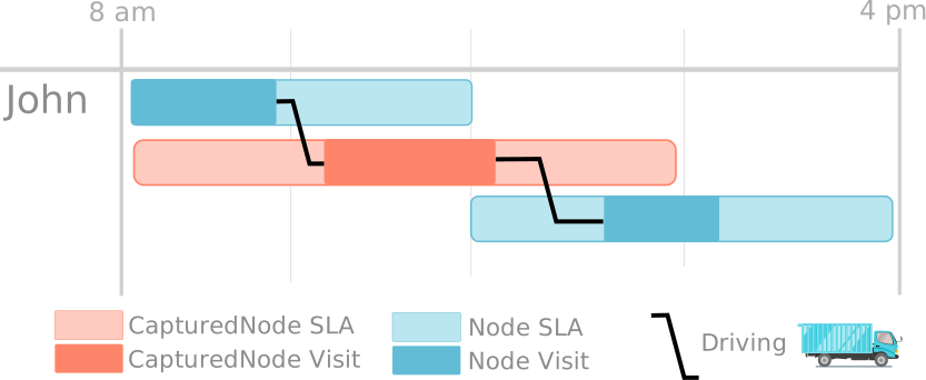
Figure: CapturedNode case 1
Case two: conflict of a CapturedNode with a node - solved by moving a node
In some cases, visiting a node before a CapturedNode would make the resource late at the CapturedNode (figure "CapturedNode case 2", left). The optimizer recognizes the potential late arrival and solves it by moving the node (right).
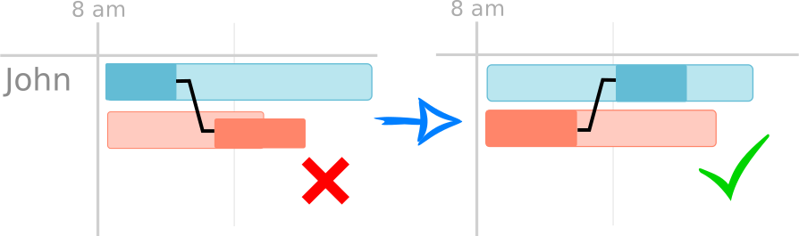
Figure: CapturedNode case 2
Case three: conflict of a CapturedNode with a node - solved via late violation at the node
Sometimes a node and a CapturedNode conflict so that only one of them can be visited without a late arrival. By definition, a CapturedNode allows no late arrival, so the node is visited late (figure "CapturedNode case 3").
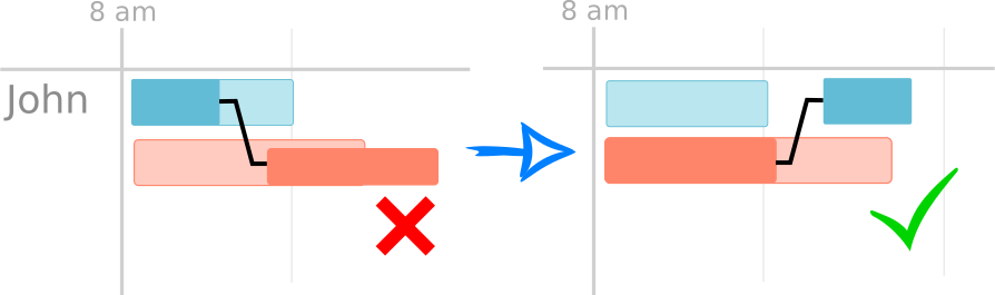
Figure: CapturedNode case 3
Case four: conflict of a CapturedNode with a node - solved by utilizing an additional resource
Larger problems usually have more resources. Often the best way to solve a late arrival is to move the conflicting node to another resource. Which node stays in the route of John depends on aspects such as driving times, required skills or the optional mandatory resource (figure "CapturedNode case 4").
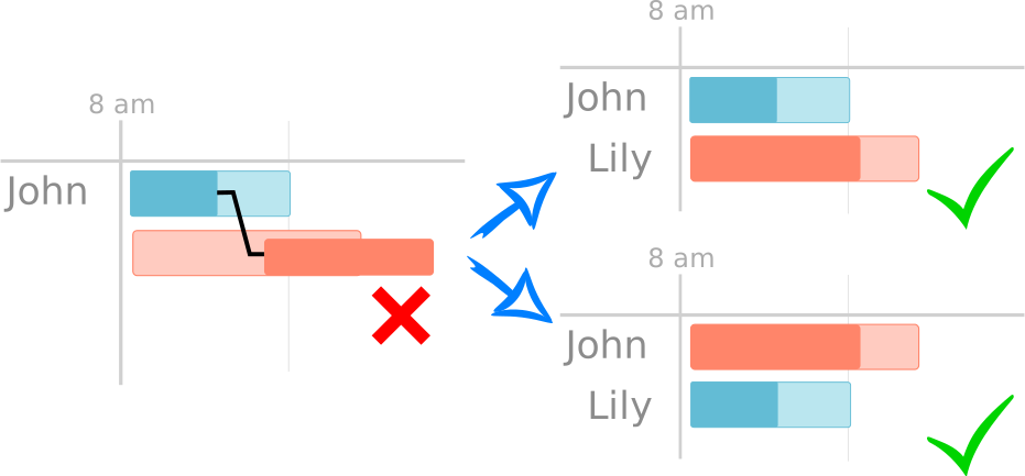
Figure: CapturedNode case 4
Case five: conflict of a CapturedNode with a node - solved by removing a CapturedNode
If John is the only resource available for two CapturedNodes that conflict with each other, the only possible solution is to remove one of the CapturedNodes. This extreme case shows the definition of a CapturedNode: its SLA cannot be violated under any circumstances. If no other solution exists, a CapturedNode contract is canceled rather than violated (figure "CapturedNode case 5").
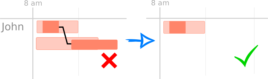
Figure: CapturedNode case 5
When to use CapturedNodes
CapturedNodes guarantee that their SLAs are matched. The architecture of the optimizer ensures this guarantee, not the optimization process itself. A CapturedNode limits the optimization, because the available optimization space shrinks. Use CapturedNodes instead of normal nodes only where a violation would lead to legal issues or other high-priority business problems, and not, for example, for a hairdressing appointment.
The optimizer is tuned to match the SLAs of normal nodes as well. CapturedNodes guarantee the match, except in the rare case of an exclusive conflict; there, skipping a CapturedNode serves as damage control.
Hard constraints - violations not allowed
The section on CapturedNodes describes hard constraints on time windows. Many business cases have other conditions that must be matched, however poor the optimization result becomes. Some jobs require a particular qualification, for example a truck driver who picks up dangerous goods. A second resource nearby, with more time and a better location but without the qualification, does not make the conditions easier to fulfill: sending the wrong resource leads to serious legal issues.
JOpt.TourOptimizer reaches solutions free of hard constraint violations through its attempt-based architecture, not through the optimization process itself. Every permutation of the order of nodes and resources leads to a new solution of the problem, and the optimizer cuts the invalid solutions out of the solution space. In return, every solution it finds is valid: not necessarily converged or at optimal cost, but without any hard constraint violation (figure "Solution space with hard constraints"). An iterative process selects the best solutions and improves them, and the solutions get better the longer the optimization runs.
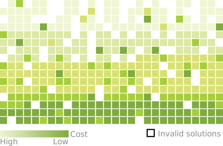
Figure: Solution space with hard constraints
Overnight stay
In JOpt.TourOptimizer, a resource can have several predefined WorkingHours; they belong to the resource and describe when it is allowed to work. Each working hours object leads to exactly one route. Time after the end of the working hours counts against the maximal working time, and the working hours are a frame for matching resources with the opening hours of the nodes, so a route can end after its working hours without a violation. Usually, a route starts and ends at the home location of the resource. Sometimes, however, a resource should be allowed to stay one or more nights in a hotel (figure "Overnight stay"). Whether a resource may stay out depends on the day and on the resource itself, and the rules can be set in detail. For example, the resource can be allowed to have a maximum of two overnight stays per week (or any other time unit), whereas Mondays and Fridays are not allowed.
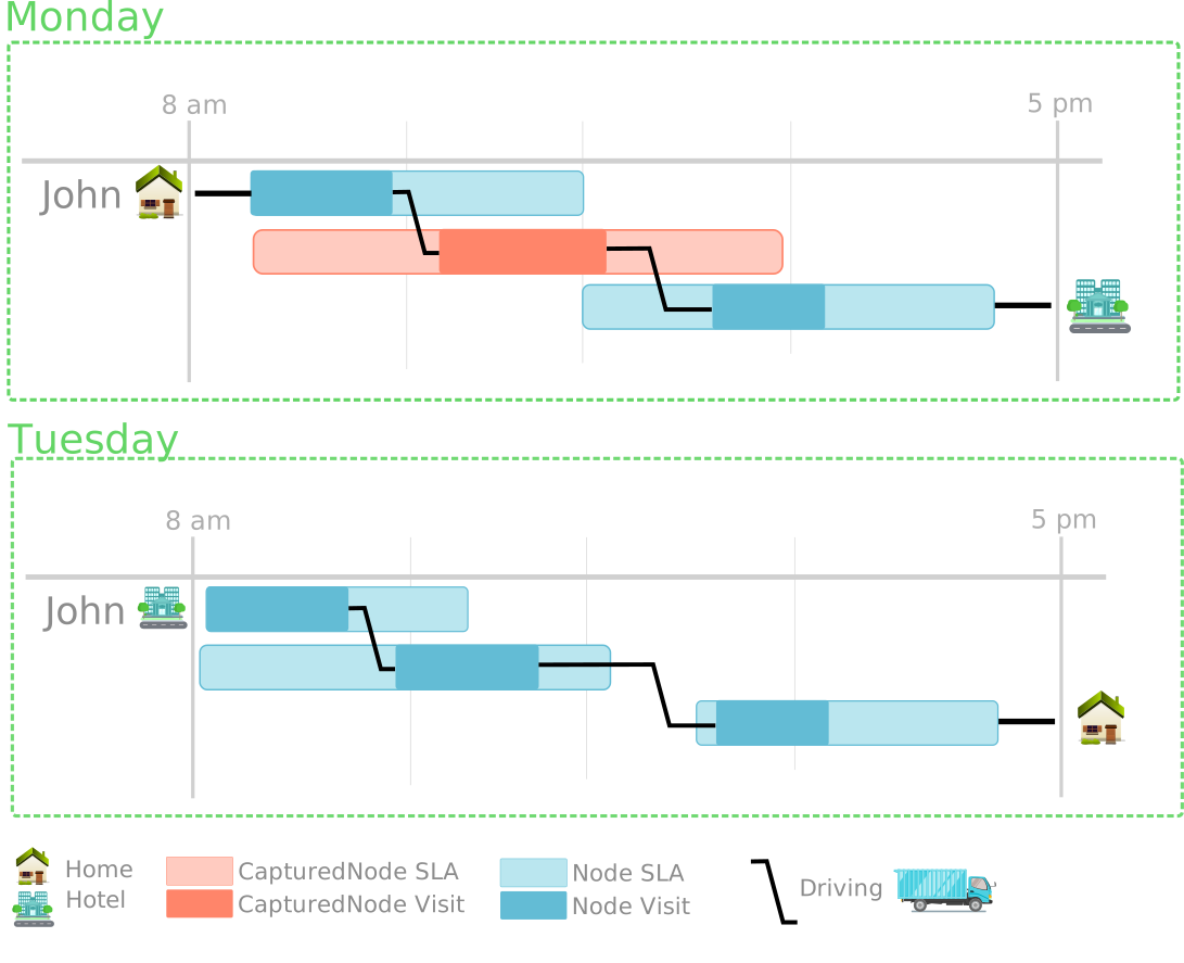
Figure: Overnight stay
Flexible start time (positive and negative)
The flexible start time lets a resource reduce idle time by starting its route later (FlexTime), or reach a node when it opens by starting the drive before its working hours (StartReductionTime). The start of the working hours becomes a bounded time window instead of a fixed time such as 8 am.
FlexTime
Each resource has a predefined start of its working hours, here 8 am. If the first node opens at 10 am, the optimizer assigns idle time to the resource by default (figure "FlexTime", top). In practice, resources are often allowed to start their workday later, depending on their schedule. In JOpt.TourOptimizer, this is called FlexTime. A custom FlexTime can be assigned to each resource and each of its working hours.
In the center of the figure, John has one hour of FlexTime. The FlexTime assigned to the working hours of a resource is hard constrained: the resource cannot use more than the assigned maximum. The idle time before the node opens is longer than the FlexTime, so John uses the full hour and reduces his idle time by one hour.
At the bottom of the figure, John has two hours of FlexTime. He uses up 90 minutes of this FlexTime to align his workday to the opening hours of the node and gets rid of the idle time completely. FlexTime has no setting that leaves the driving time out: the FlexTime used is the time John would otherwise wait at the node. The driving-time setting belongs to StartReductionTime (setMaxRouteStartReductionTime with true), see below.
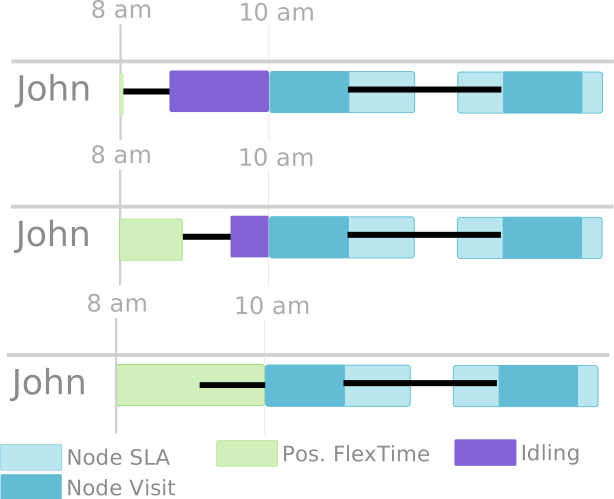
Figure: FlexTime
setWaitOnEarlyArrival(false), read with isWaitOnEarlyArrival. The result reports such an early start as an EARLY violation with a cost. The wait on early arrival example page shows it.StartReductionTime
StartReductionTime is the counterpart of FlexTime. Assume that a node opens at 8 am and that the resource John also starts working at 8 am. John needs 30 minutes to drive to the first node, so he would reach the node and start working at 8:30. With a StartReductionTime of up to one hour, defined as "only allowed to be used for driving", John starts driving at 7:30 am and reaches the node ready to work at 8 am (figure "StartReductionTime").
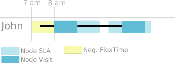
Figure: StartReductionTime
The figure "StartReductionTime with four resources" shows four resources at the top. There are no violations, but the Gantt chart looks irregular because of the driving times. With StartReductionTime (bottom), the first nodes of the routes line up and are visited when their opening hours begin. The exception is Bob: his maximal StartReductionTime is not long enough to reach his first node when it opens. Like FlexTime, StartReductionTime is hard constrained and cannot be exceeded.
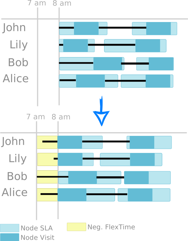
Figure: StartReductionTime with four resources
Combining FlexTime and StartReductionTime
FlexTime and StartReductionTime can be combined. The start of the working hours of a resource then becomes a flexible time window, and the optimizer uses it as the circumstances of each workday require.
Optional nodes
Usually, every node creates cost: each additional node in a solution increases the total cost. In pickup and delivery scenarios, however, an optional node can reduce the cost. The optimizer decides whether visiting an optional node lowers the total cost. A node becomes optional with setIsOptional(true).
In a waste management scenario, optional nodes (here: waste deposits) give the resource an opportunity to dump the collected waste. An overload is penalized, so unloading the waste at an optional node before the truck is full avoids the overload cost.
The figure "Optional nodes" shows two routes, starting in Stuttgart and in Ulm. On the route from Stuttgart, the resource picks up 20 units of waste at the first node and another 30 units at the second node. Assume that the maximal loading capacity of the resource is 50 units: it cannot pick up more waste without being overloaded. By visiting an optional node, it unloads the waste before it visits the next node. The optional node at Freiburg is not visited.
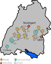
Figure: Optional nodes
Pickup and delivery (PND) - manufacturing planning
In a PND problem, a customer (node) requests or supplies goods, and a resource tries to serve these demands. Solving a PND problem means an optimal exchange of goods between the parties, free of violations.
This section shows how the PND module of JOpt.TourOptimizer plans the manufacturing of goods in addition to their transport. To our best knowledge, no other routing engine we checked offers this as a built-in feature: there, supply and demand quantities are input values.
Example: a bakery chain plans its production
In this manufacturing planning task, a bakery company has two production sites for bread, Bakery Aachen and Bakery Cologne. The two sites are in different cities, and each has one employee (a resource) who supplies stores (nodes) with trays of bread. Each production site may supply each store. The truck of a resource can load a maximum of 20 trays of bread. The figure "Bakery setup" shows the setup.
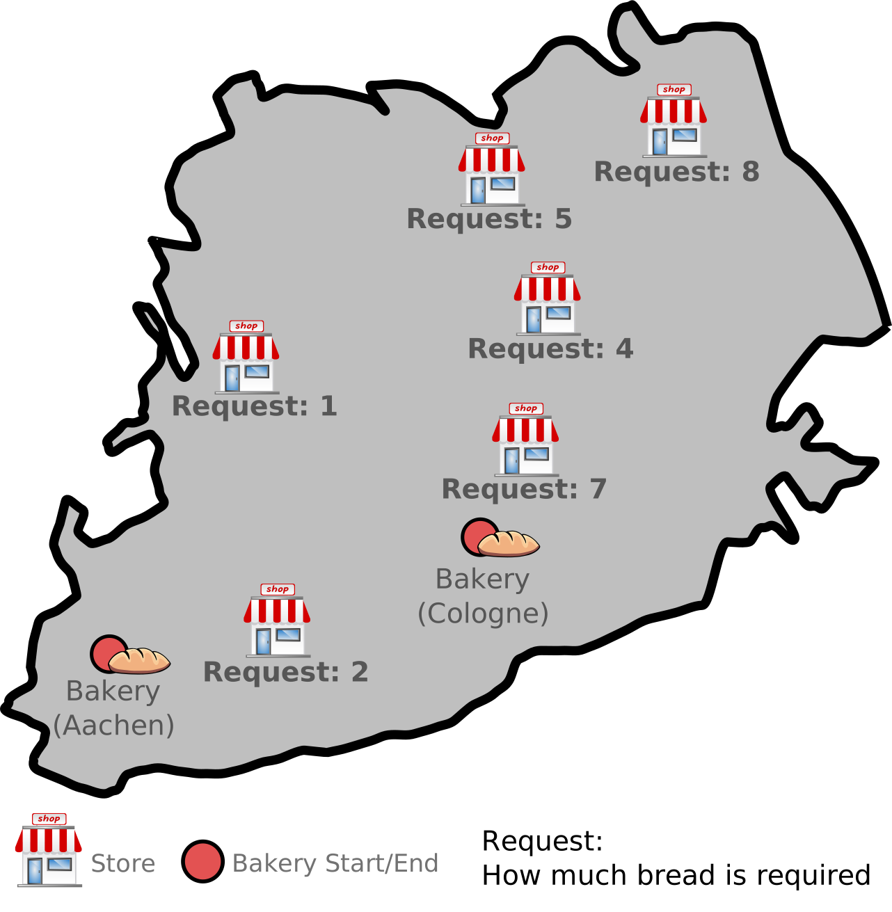
Figure: Bakery setup
The bakery does not want to waste bread, and it wants an optimal route (time windows kept, a short total distance). So the optimizer does the manufacturing planning: the optimizer decides how much bread each production site produces.
For this, each production site gets a factory for bread, a supply node with a flexible supply. The supply nodes are not optional nodes: both are on the plan, and each adjusts the number of trays of bread it produces, based on what is best for the overall optimization problem. For simplicity, each supply node is at the start position of the truck of its site, in Aachen and in Cologne. In general, factories can be located at any position.
The figure "Bakery result" shows the optimized result: Bakery Aachen produces 10 trays of bread in its factory, and Bakery Cologne produces 17 trays.
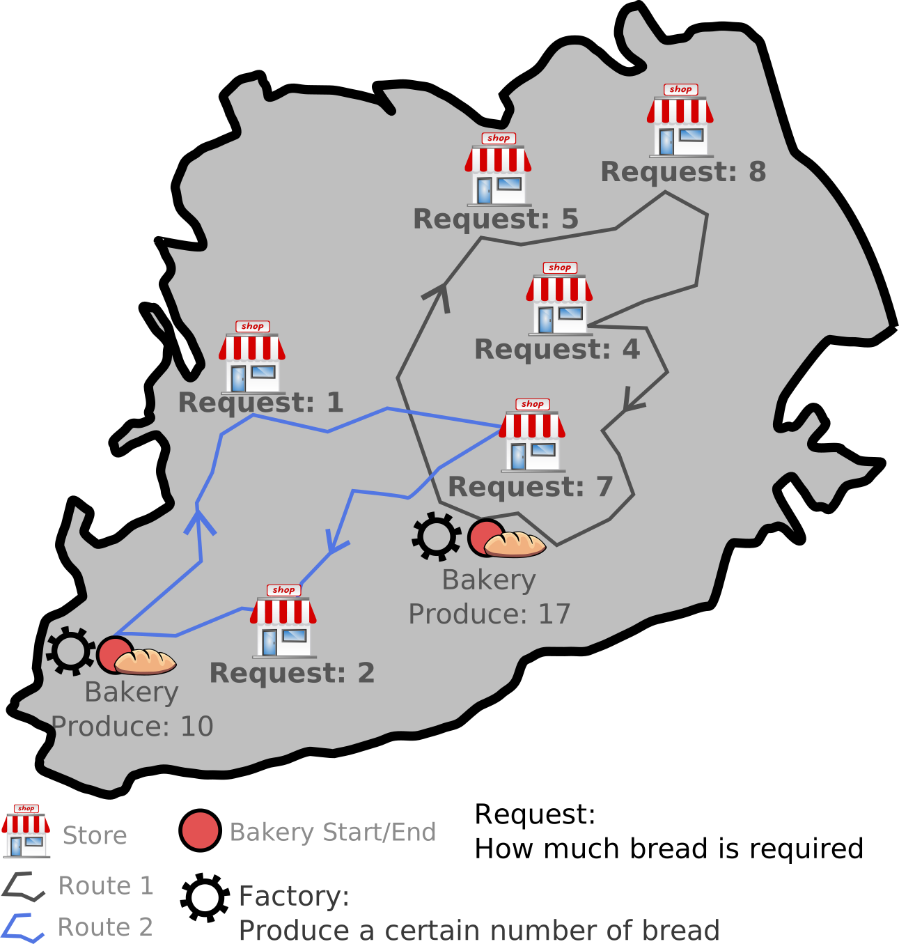
Figure: Bakery result
This task is small and easy to solve. The concept pays off with mixed pickup and delivery problems and with problems that have many nodes and several constraints.
Defining territories via ZoneCodes
Resources are often restricted: they are bound to territories, or a customer prefers a particular resource. The territories of the resources can also change from day to day. For these problems, JOpt has ZoneCodes, which work similar to postcodes.
ZoneCodes attached to resources and nodes tell the optimizer which resources may visit the nodes with matching ZoneCodes. For fine control, the ZoneCodes are defined for each working hours of a resource, and a resource can be allowed to visit several ZoneCodes.
Each node gets one or more ZoneCodes. Several ZoneCodes on one node make sense when the node lies on a territory border; the optimizer then decides which resource visits it at the smallest additional cost. The figure "ZoneCodes" shows a typical setup.
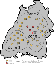
Figure: ZoneCodes
Compared with abstract territories, ZoneCodes let you define fine-grained and precise territories for the needs of each customer; small territories can lie within large ones, for example. ZoneCodes can also be hard constraints if necessary.
AutoFilter
In an optimization, a few nodes can cause most of the violations. One node may be so far away from the home locations of all resources that no resource can visit it in time. The number of nodes can be too high to fit into the available working hours of the resources. Or too many nodes demand a particular resource as their preferred resource.
During an optimization run, JOpt.TourOptimizer creates a large number of parallel solutions; each solution is a full schedule of all nodes and all resources. The AutoFilter analyzes each solution for the nodes that caused a violation.
The figure "AutoFilter" shows two solutions for one route. One solution turns right, the other turns left. As a result, node D is visited late in solution one and node A in solution two. The AutoFilter assesses both solutions and assigns penalty points to node A and to node D.
During the optimization, the nodes collect these penalty points over many solutions. The AutoFilter excludes the nodes that are prone to cause violations: if the penalty points of a node become too high compared with the number of solutions in which it shows no violation, the node is filtered out at the next AutoFilter execution; the AutoFilter usually removes nodes in chunks over several rounds. Custom filter reasons can be set, and so can the margins for being filtered out. Particular reasons, such as late or early arrivals, can be set to filter a node without that ratio, in the strict mode of the last AutoFilter execution. Individual nodes can be protected from being filtered out at all.
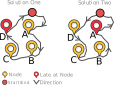
Figure: AutoFilter
Custom solution
At the start of an optimization run, a deterministic construction algorithm creates a first starting solution, which the following steps optimize further. Such a solution helps, because it narrows the space in which desirable solutions are searched.
Because it is deterministic, the construction algorithm is less flexible than the optimization algorithms that follow it. For particular use cases, either a custom construction algorithm can be defined (contact us), or you construct a starting solution on your own and provide it at the start with setInitialEntity.
JOpt saves an optimization state as a human-readable JSON definition. A saved state can be loaded as the start of a custom solution; the CreateCustomSolutionFromJSON example page shows where your own construction logic plugs in.
Open Assessor
JOpt.TourOptimizer has many predefined restrictions, but end customers sometimes require restrictions of their own. The Open Assessor injects such custom restrictions into the optimization. The two conditions below show how it works.
Custom condition on node level
An end customer requests that each node is visited as early as possible within its opening hours. Take a problem with two nodes: node A is open from 8 am to 5 pm, and node B from 9 am to 5 pm. A resource needs one hour to drive to either node (figure "Open Assessor at node level").
By default, the optimizer can schedule node A or node B first at exactly the same cost: in both orders the first node is reached at 9 am, and no late, early or idle time arises.
The customer, however, prefers visits as early as possible within the opening hours. Node A has been open for one hour when the resource arrives, so node A should be visited before node B (figure, left).
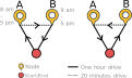
Figure: Open Assessor at node level
A custom restriction tells the optimizer that a particular order of nodes is preferred.
In CustomNodeLevelRestrictionExample on GitHub, all nodes whose ids start with a capital "M" should be visited before 11 am; otherwise a penalty applies.
Custom condition on route level
Custom restrictions also work at route level. For example, you can tell the optimizer to prefer routes with an odd number of nodes (figure "Open Assessor at route level"). With the Open Assessor, you formulate this restriction and inject it into the optimization.
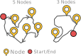
Figure: Open Assessor at route level
Clustering construction
JOpt.TourOptimizer uses a multi-algorithm solving strategy: several algorithms run in direct succession, and the output of one algorithm is the input of the next.
By default, a deterministic construction algorithm, SmartConstructionAlgo, first creates an initial starting solution (the working solution). In theory, a constructed starting solution is not necessary, but it helps the following non-deterministic optimization algorithms to converge faster to a better solution. With the same computing power, the expected quality of the solution is much higher when construction is used.
SmartConstructionAlgo creates feasible or near-feasible solutions for different problem scenarios. Its result is also used as an approximate solution for end customers before any further optimization steps. The Clustering during construction feature guide describes SmartConstructionAlgo and shows construction results, and the clustering example page explains the clustering examples.
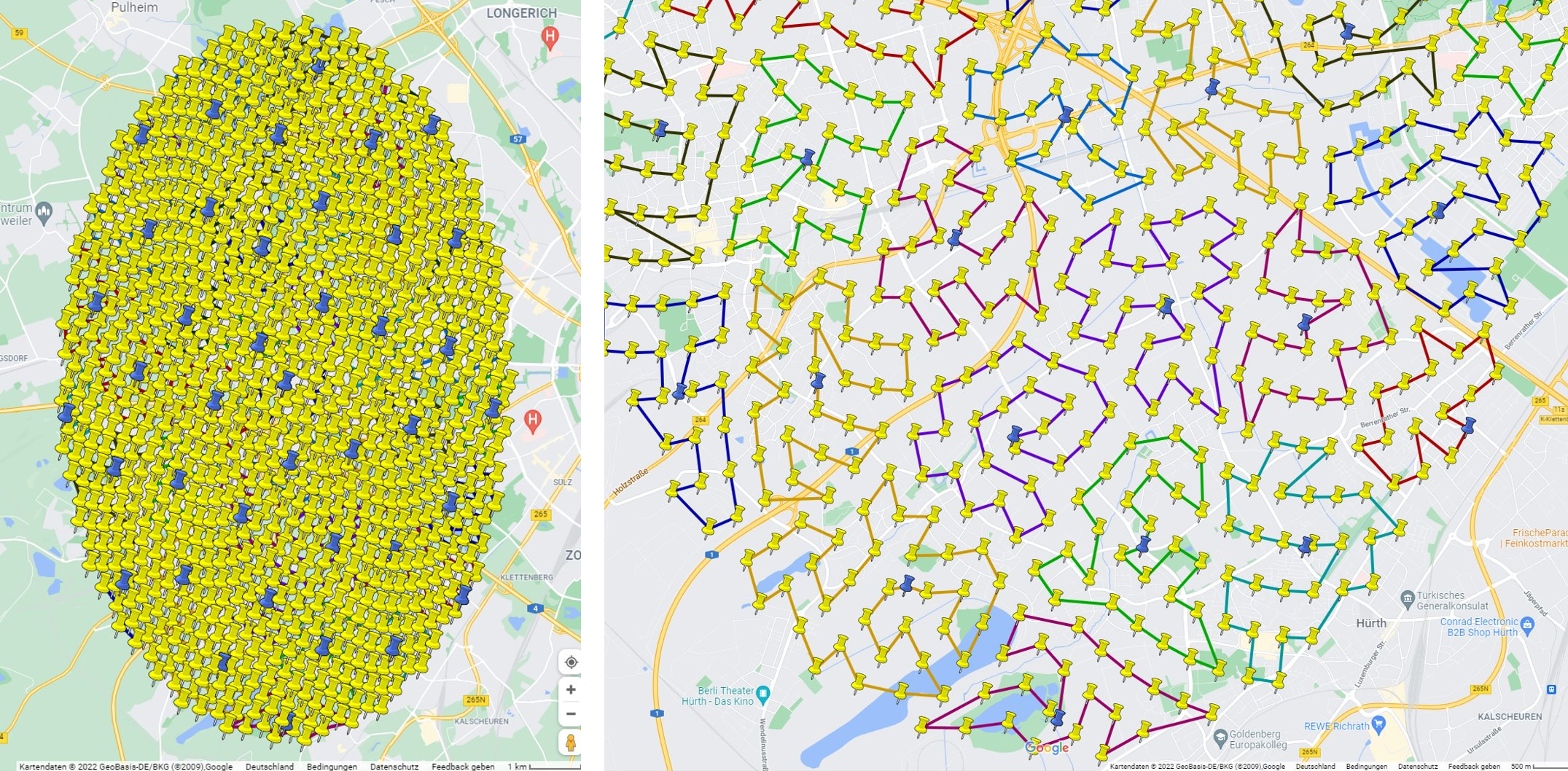
Figure: Phyllotaxis solved by construction
Related pages
- Feature list: the features by topic, with a level for each feature
- Feature guides: one guide per feature, with the code and the properties
- Pillar nodes: CapturedNodes, their node classes and the conflict cases
- Overnight stay: stay nodes, stay-out policies and their restrictions
- Flexible start time: FlexTime and StartReductionTime in Java
- Pickup and delivery: loads, depots, capacities and the depot reports
- Manufacturing planning: production planning with flexible loads
- ZoneCodes and territories: territories per working hours, hard or soft
- AutoFilter: the AutoFilter, its properties and its margins
- Open Assessor: custom costs, violations and scoring at node level and route level
- Clustering during construction: SmartConstructionAlgo, the construction algorithm that runs by default, and figures of construction results
- Java-TourOptimizer-Examples: the Java examples on GitHub, which cover more features than this page
- Contact: questions about a feature that you are missing
Authors
DNA Evolutions GmbH
Added: 2026-01-03 (JOpt core 7.5.2-j17) | Last updated: 2026-10-23
Zone crossing penalization
How JOpt adds a cost when a route moves from one zone into another, with a global multiplier and optional multipliers per direction.
REST-Clients for JOpt.TourOptimizer
JOpt.TourOptimizer can be containerized using Docker, which means that it can be run as a container on any system that has Docker installed. This allows for easy deployment and scaling of the service.