First optimization with JOpt for Java

This tutorial sets up a complete optimization problem in Java, step by step, and combines the basic parts of every optimization setup for JOpt.TourOptimizer. In the problem, one resource called Jack visits several nodes across Germany. At the end, the tutorial explains how to read the result. Read the Basic elements tutorial first.
Table of contents
- Before you start
- Set up the example file
- (1) Adding properties
- (2) Adding nodes
- (3) Adding resources
- (4) Attaching to observables
- (5) Starting the optimization and presenting the result
- Analyzing the result
- Get the example
- Related pages
Before you start
- JOpt in your Java project, as a Maven dependency or as a JAR file; see Getting started.
- A JDK in the version that the examples pom sets.
- A license if your optimization has more elements than JOpt allows without one: License guide: element limits.
Set up the example file
Create a file FirstOptimizationExample.java in the package com.dna.jopt.touroptimizer.java.examples.basic.firstoptimization_01. The class extends Optimization and has a main() and an example() method. The code below is the starting point, with all imports that the tutorial needs. The numbered comments (1) to (5) in example() mark the parts that the next steps fill in.
Show or hide the code
package com.dna.jopt.touroptimizer.java.examples.basic.firstoptimization_01;

import static javax.measure.MetricPrefix.KILO;
import static tech.units.indriya.unit.Units.METRE;
import static java.time.Month.MAY;

import tech.units.indriya.quantity.Quantities;

import javax.measure.Quantity;
import javax.measure.quantity.Length;

import java.time.Duration;
import java.time.ZoneId;
import java.time.ZonedDateTime;
import java.util.ArrayList;
import java.util.List;
import java.util.Properties;
import java.util.concurrent.CompletableFuture;
import java.util.concurrent.ExecutionException;

import com.dna.jopt.framework.body.IOptimization;
import com.dna.jopt.framework.body.Optimization;
import com.dna.jopt.framework.exception.caught.InvalidLicenceException;
import com.dna.jopt.framework.outcomewrapper.IOptimizationResult;
import com.dna.jopt.member.unit.hours.IWorkingHours;
import com.dna.jopt.member.unit.hours.IOpeningHours;
import com.dna.jopt.member.unit.hours.WorkingHours;
import com.dna.jopt.member.unit.hours.OpeningHours;
import com.dna.jopt.member.unit.node.INode;
import com.dna.jopt.member.unit.node.geo.TimeWindowGeoNode;
import com.dna.jopt.member.unit.resource.CapacityResource;
import com.dna.jopt.member.unit.resource.IResource;

public class FirstOptimizationExample extends Optimization {

    public static void main(String[] args) throws InterruptedException, ExecutionException, InvalidLicenceException {
        new FirstOptimizationExample().example();
    }

    public void example() throws InterruptedException, ExecutionException, InvalidLicenceException {
      // Will be filled out as part of this tutorial

      // Setting properties, adding all elements, and attaching to observables
      //    (1) Adding properties

      //    (2) Adding nodes

      //    (3) Adding resources

      //    (4) Attach to Observables

      // Starting the optimization via Completable Future
      // and presenting the result
      //    (5) Starting the optimization and presenting the result

    }


}
(1) Adding properties
JOpt can start without any properties. To get a fully functional optimization with a convincing outcome, settings help a lot; the optimization properties page lists the property keys by category, with their defaults. The following static method adds two settings to an optimization instance. The next part of this step adds the method to the example file.
  private static void addProperties(IOptimization opti) {

     // Create an empty properties object
    Properties props = new Properties();

    props.setProperty("JOpt.Algorithm.PreOptimization.SA.NumIterations", "10000");
    props.setProperty("JOptExitCondition.JOptGenerationCount", "2000");

    // Adding the properties to the optimization
    opti.addElement(props);
  }
What the two properties set
JOpt.Algorithm.PreOptimization.SA.NumIterations: the number of iterations of the simulated annealing pre-optimization. The tutorial sets 10,000 iterations; a real problem usually needs many more. The default is on the optimization properties page.JOptExitCondition.JOptGenerationCount: the number of generations of the genetic evolution, one of the standard algorithms. It sets how many generations run one after the other. The value should be in the order of several thousand. The default is on the same page.
Call addProperties() from example()
Copy the method addProperties() into the class body and add FirstOptimizationExample.addProperties(this); in section (1):
Show or hide the code
    ...
    public void example() throws InterruptedException, ExecutionException, InvalidLicenceException {

      // Will be filled out as part of this tutorial

      // Setting properties, adding all elements, and attaching to observables
      //    (1) Adding properties
      FirstOptimizationExample.addProperties(this);

      //    (2) Adding nodes

      //    (3) Adding resources

      //    (4) Adding resources

      //    (5) Attach to Observables

      // Starting the optimization via Completable Future
      // and presenting the result
      //    (6) Starting the optimization and presenting the result

    }

    private static void addProperties(IOptimization opti){
        ...
    }
    ...
Optimization, the argument this refers to an optimization instance.(2) Adding nodes
This step defines the nodes to visit. Each node has a different position in Germany. To keep the tutorial simple, all nodes have the same opening hours, visit duration and importance. These are sample values:
- Opening hours: the 6th and the 7th of May, from 8 in the morning to 5 in the afternoon
- Visit duration: 20 minutes
- Importance: 1
The static method addNodes(IOptimization opti) adds each node to the optimization on its own, with opti.addElement(someNode);.
Show or hide the code
 private static void addNodes(IOptimization opti) {

    List<IOpeningHours> weeklyOpeningHours = new ArrayList<>();
    weeklyOpeningHours.add(
        new OpeningHours(
            ZonedDateTime.of(2020, MAY.getValue(), 6, 8, 0, 0, 0, ZoneId.of("Europe/Berlin")),
            ZonedDateTime.of(2020, MAY.getValue(), 6, 17, 0, 0, 0, ZoneId.of("Europe/Berlin"))));

    weeklyOpeningHours.add(
        new OpeningHours(
            ZonedDateTime.of(2020, MAY.getValue(), 7, 8, 0, 0, 0, ZoneId.of("Europe/Berlin")),
            ZonedDateTime.of(2020, MAY.getValue(), 7, 17, 0, 0, 0, ZoneId.of("Europe/Berlin"))));

    Duration visitDuration = Duration.ofMinutes(20);

    int importance = 1;

    // Define some nodes
    INode koeln =
        new TimeWindowGeoNode("Koeln", 50.9333, 6.95, weeklyOpeningHours, visitDuration, importance);
    opti.addElement(koeln);

    INode essen =
        new TimeWindowGeoNode("Essen", 51.45, 7.01667, weeklyOpeningHours, visitDuration, importance);
    opti.addElement(essen);

    INode dueren =
        new TimeWindowGeoNode("Dueren", 50.8, 6.48333, weeklyOpeningHours, visitDuration, importance);
    opti.addElement(dueren);

    INode nuernberg =
        new TimeWindowGeoNode("Nuernberg", 49.4478, 11.0683, weeklyOpeningHours, visitDuration, importance);
    opti.addElement(nuernberg);

    INode heilbronn =
        new TimeWindowGeoNode("Heilbronn", 49.1403, 9.22, weeklyOpeningHours, visitDuration, importance);
    opti.addElement(heilbronn);

    INode wuppertal =
        new TimeWindowGeoNode("Wuppertal", 51.2667, 7.18333, weeklyOpeningHours, visitDuration, importance);
    opti.addElement(wuppertal);

    INode aachen =
        new TimeWindowGeoNode("Aachen", 50.775346, 6.083887, weeklyOpeningHours, visitDuration, importance);
    opti.addElement(aachen);
  }
Call addNodes() from example()
Copy the method addNodes() into the class body and add FirstOptimizationExample.addNodes(this); in section (2), as in (1) Adding properties.
(3) Adding resources
Each node needs to be visited by a resource. In this tutorial, it is one resource called "Jack from Aachen". Jack has these sample values:
- Working hours: the 6th and the 7th of May, from 8 in the morning to 5 in the afternoon
- Maximal working time (per working hours): 9 hours
- Maximal distance (per working hours): 1200 km
- Start location: Aachen (latitude 50.775346, longitude 6.083887)
The static method addResources(IOptimization opti) adds Jack to the optimization with opti.addElement(jack);.
Show or hide the code
   private static void addResources(IOptimization opti) {

    List<IWorkingHours> workingHours = new ArrayList<>();
    workingHours.add(
        new WorkingHours(
            ZonedDateTime.of(2020, MAY.getValue(), 6, 8, 0, 0, 0, ZoneId.of("Europe/Berlin")),
            ZonedDateTime.of(2020, MAY.getValue(), 6, 17, 0, 0, 0, ZoneId.of("Europe/Berlin"))));

    workingHours.add(
        new WorkingHours(
            ZonedDateTime.of(2020, MAY.getValue(), 7, 8, 0, 0, 0, ZoneId.of("Europe/Berlin")),
            ZonedDateTime.of(2020, MAY.getValue(), 7, 17, 0, 0, 0, ZoneId.of("Europe/Berlin"))));

    Duration maxWorkingTime = Duration.ofHours(9);
    Quantity<Length> maxDistanceKmW = Quantities.getQuantity(1200.0, KILO(METRE));

    IResource jack =
        new CapacityResource(
            "Jack from Aachen", 50.775346, 6.083887, maxWorkingTime, maxDistanceKmW, workingHours);
    opti.addElement(jack);
  }
Call addResources() from example()
Copy the method addResources() into the class body and add FirstOptimizationExample.addResources(this); in section (3), as in (1) Adding properties.
(4) Attaching to observables
To follow the running optimization and to get its warnings, statuses and error messages, you subscribe to its events. JOpt provides several ReplaySubjects for this.
The static method attachToObservables(IOptimization opti) subscribes to the progress, warning, status and error events:
Show or hide the code
  private static void attachToObservables(IOptimization opti) {

    opti.getOptimizationEvents()
        .progressSubject()
        .subscribe(
            p -> {
              System.out.println(p.getProgressString());
            });

    opti.getOptimizationEvents()
        .warningSubject()
        .subscribe(
            w -> {
              System.out.println(w.toString());
            });

    opti.getOptimizationEvents()
        .statusSubject()
        .subscribe(
            s -> {
              System.out.println(s.toString());
            });

    opti.getOptimizationEvents()
        .errorSubject()
        .subscribe(
            e -> {
              System.out.println(e.toString());
            });
  }
Each lambda body prints its event.
Call attachToObservables() from example()
Copy the method attachToObservables() into the class body and add FirstOptimizationExample.attachToObservables(this); in section (4), as in (1) Adding properties.
(5) Starting the optimization and presenting the result
This step runs the optimization. First, opti.startRunAsync() returns a completable future for the optimization result. In the next step, we have to perform a blocking call via get() on the future object, resulting in the start of the optimization. When the optimization is done, the method prints the optimization result.
The static method startAndPresentResult(IOptimization opti) starts the optimization and prints the result:
private static void startAndPresentResult(IOptimization opti) throws
    InvalidLicenceException, InterruptedException, ExecutionException {

    // Extracting a completable future for the optimization result
    CompletableFuture<IOptimizationResult> resultFuture = opti.startRunAsync();

    // It is important to block the call, otherwise optimization will be terminated
    IOptimizationResult result = resultFuture.get();

    // Presenting the result
    System.out.println(result);
  }
Call startAndPresentResult() from example()
Copy the method startAndPresentResult() into the class body and add FirstOptimizationExample.startAndPresentResult(this); in section (5), as in (1) Adding properties.
After this last part, the example() method looks as follows:
Show or hide the code
  public void example() throws InterruptedException, ExecutionException, InvalidLicenceException {

    // Will be filled out as part of this tutorial

    // Setting properties, adding all elements, and attaching to observables
    //    (1) Adding properties
    FirstOptimizationExample.addProperties(this);

    //    (2) Adding nodes
    FirstOptimizationExample.addNodes(this);

    //    (3) Adding resources
    FirstOptimizationExample.addResources(this);

    //    (4) Attach to Observables
    FirstOptimizationExample.attachToObservables(this);

    // Starting the optimization via Completable Future
    // and presenting the result
    //    (5) Starting the optimization and presenting the result
    FirstOptimizationExample.startAndPresentResult(this);

  }
Run the example
When you run the example, the console shows the output of the optimization:
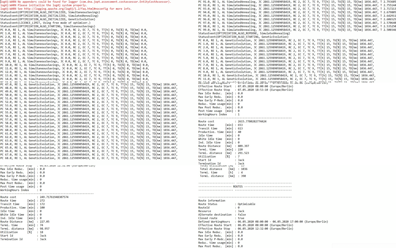
Analyzing the result
The example prints the result with the toString() method of the class OptimizationResult. You can also take the result object itself and process it as you need.
Analyzing the result header
This part looks at the header of the result first, then at a single route and its node results. The header condenses the route results into overview numbers. In this sample run, for example, all resources together spend about 15 hours (driving, working, idling):
-------------------------------- --------------------------
--------------------- RESULTS -----------------------------
----------------- -----------------------------------------
 Number of Route         : 2
 Number of Route (sched.): 2
 Total Route Elements    : 8
 Total cost              : 2865.4956477605183
-----------------------------------------------------------
 Total time        [h]   : 15
 Total idle time   [h]   : 0
 Total prod. time  [h]   : 2
 Total tran. time  [h]   : 13
 Total distance    [km]  : 1036
 Termi. time       [h]   : 4
 Termi. distance   [km]  : 390
- Number of Route: The number of routes of the problem. Each route is one
workingHoursobject of one resource. Here, the one resource Jack has two working hours, so there are two routes. - Number of Route (sched.): The number of scheduled routes, that is, routes that carry nodes.
- Total Route Elements: The number of elements, nodes and resources together.
- Total cost: JOpt uses a cost assessment to decide which of two results is better. Each result gets an abstract cost value (the figure of merit); a lower cost means a better result.
- Total time: The total time spent by all resources (driving, working, idling).
- Total idle time: The total time the resources wait, for example because a node is closed and opens in 30 minutes.
- Total prod. time: The total productive time, the time the resources work at the nodes.
- Total tran. time: The total time the resources need to move from one location to another.
- Total distance: The total distance the resources move from one location to another.
- Termi. time: The total time the resources need from the last node of a route to their home locations.
- Termi. distance: The total distance the resources move from the last node of a route to their home locations.
Analyzing a route result header
Each route has its own header with condensed route information. Some parts are left out here for simplicity:
-----------------------------------------------------------
Route information
RouteId                : 0
Resource               : Jack from Aachen
Closed route           : true
Defined WorkingHours   : 06.05.2020 08:00:00 - 06.05.2020 17:00:00 (Europe/Berlin)
Effective Route Start  : 06.05.2020 08:00:00 (Europe/Berlin)
Effective Route Stop   : 06.05.2020 12:32:00 (Europe/Berlin)
WorkingHours Index     : 0
-----------------------------------------------------------
Route cost             : 249.71761948307574
Route time       [min] : 272
Transit time     [min] : 172
Productive. time [min] : 100
Idle time        [min] : 0
Route Distance   [km]  : 227.05
Route Emission [kgCO2] : 85.59
Termi. time      [min] : 0
Termi. distance  [km]  : 0.0
Utilization      [%]   : 18
Start Id               : Jack from Aachen
Termination Id         : Jack from Aachen
- Route id: Each route has a unique route id, an integer value.
- Resource: The resource that owns the route.
- Closed route: Each route has a start and a termination element. Usually, both are the home location of the resource. A route that is not closed has no termination element; its last node becomes the effective termination element.
- Defined WorkingHours: The working hours of the resource that belong to this route.
- Effective Route Start: The time the resource starts working. By default, this is the start of the working hours.
- Effective Route Stop: The time the resource is done with the route.
- WorkingHours Index: A resource can carry several working hours as a list. Each route belongs to one entry of that list.
- Route cost: The result of the cost assessment for this route.
- Route time: The route's share of "Total time".
- Transit time: The route's share of "Total tran. time".
- Productive. time: The route's share of "Total prod. time".
- Idle time: The route's share of "Total idle time".
- Route Distance: The route's share of "Total distance".
- Route Emission: The emitted CO2 of the route, in kilograms.
- Termi. time: The route's share of "Termi. time" in the result header.
- Termi. distance: The route's share of "Termi. distance" in the result header.
- Start Id: The id of the start element of the route.
- Termination Id: The id of the termination element of the route.
Analyzing a route
A route is an ordered list of nodes that belongs to one resource and one working hours object. For each visited node, the planned arrival, the departure and any violations are the most interesting part of the optimization result:
0.0 Dueren /
Arrival: 06.05.2020 08:21:21 (Europe/Berlin) ,
Departure: 06.05.2020 08:41:21 (Europe/Berlin) /
Duration: 20 [min] /
Driving: 21.36 [min], 28.201 [km]

0.1
Koeln /
Arrival: 06.05.2020 09:08:36 (Europe/Berlin) ,
Departure: 06.05.2020 09:28:36 (Europe/Berlin) /
Duration: 20 [min] /
Driving: 27.25 [min], 35.966 [km]

0.2
Wuppertal /
Arrival: 06.05.2020 09:59:17 (Europe/Berlin) ,
Departure: 06.05.2020 10:19:17 (Europe/Berlin) /
Duration: 20 [min] /
Driving: 30.67 [min], 40.49 [km]

0.3
Essen /
Arrival: 06.05.2020 10:37:02 (Europe/Berlin) ,
Departure: 06.05.2020 10:57:02 (Europe/Berlin) /
Duration: 20 [min] /
Driving: 17.75 [min], 23.433 [km]

0.4
Aachen /
Arrival: 06.05.2020 12:12:00 (Europe/Berlin) ,
Departure: 06.05.2020 12:32:00 (Europe/Berlin) /
Duration: 20 [min] /
Driving: 74.97 [min], 98.957 [km]
The following table takes the result for Koeln (Cologne) apart:
| Variables | Result values for Koeln |
|---|---|
| "RouteId" . "VisitingIndex" | 0.1 |
| "Element Id" | Koeln |
Arrival (ZonedDateTime) | Arrival: 06.05.2020 09:08:36 (Europe/Berlin) |
Departure (ZonedDateTime) | Departure: 06.05.2020 09:28:36 (Europe/Berlin) |
| Visit duration | Duration: 20 min |
| Driving time from the previous element | Driving: 27.25 min |
| Driving distance from the previous element | Driving: 35.966 km |
Get the example

The example that this tutorial describes is FirstOptimizationExample.java on GitHub. It is part of Java-TourOptimizer-Examples, a collection of Java examples and a working Maven project that you can clone and use as a base for starting with JOpt.TourOptimizer.
Related pages
- Basic elements: the nodes, resources and properties that this tutorial combines
- First optimization example: the example page of
FirstOptimizationExample - Basic examples: more examples at the basic level
- Optimization properties: the property keys by category, with their defaults
Authors
DNA Evolutions GmbH
Added: 2026-01-03 (JOpt core 7.5.2-j17) | Last updated: 2026-10-19