Clustering during construction

JOpt.TourOptimizer builds its starting solution with a construction algorithm before the optimization algorithms run. This guide describes the multi-dimensional clustering of SmartConstructionAlgo, the construction algorithm that runs by default, and shows construction results on three examples. It is written for developers who want to understand or inspect the starting solution; How JOpt.TourOptimizer works explains the algorithms that follow it.

What it does

JOpt.TourOptimizer uses a multi-algorithm solving strategy: different algorithms run in direct succession to solve a tour optimization problem, and the output of one algorithm is the input of the next.

By default, the first step is a deterministic construction algorithm that creates an initial starting solution (working solution). In theory, a constructed starting solution is not necessary, but it helps the subsequent non-deterministic optimization algorithms to converge faster to a better solution.

With the same processing power, the expected quality of the solution is highly improved when construction is used.

This guide shows examples of the output of SmartConstructionAlgo, the clustering construction algorithm that DNA Evolutions developed for the requirements below.

When no construction algorithm is chosen, JOpt.TourOptimizer runs SmartConstructionAlgo (ConstructionOptimizationAlgorithm.SMART_CONSTR_ALGO), which builds the starting solution from clusters. It is heavily used worldwide in production.

Requirements of the algorithm

SmartConstructionAlgo is developed to fulfil the following requirements:

• Fast: The runtime should be on a scale of seconds, up to a low minute scale, even for big problem sets (> 1000 elements).
• Robust: No matter how the input data looks, the construction result should be meaningful and provide a feasible or near-feasible solution.
• Multi-dimensional: Data clustering often uses one specific merit figure. In tour optimization problems, the distance between elements is often used to define clusters. However, the WorkingHours of resources and the OpeningHours of nodes play a critical role in deciding which nodes belong to a cluster and which resource (or collection of resources) should own that cluster. Constraints can also exclude a resource from visiting a node.
• Dynamic: The user input alone defines the number of resources and nodes (and all their properties), so the number of clusters cannot be determined a priori. The algorithm alone decides on the number of clusters and their population.

Working principle

The basic idea of SmartConstructionAlgo is a multi-stage attempt. The algorithm uses strategies from well-known clustering algorithms like K-Means, DBSCAN and hierarchical clustering, and tries to overcome some of their drawbacks for tour optimization problems. For example, the algorithm is designed to handle single-depot, multi-depot and effective multi-depot problems.

Summarized working principle:

1. Collect Resources and Nodes and calculate free path lengths between them to define an approximate local size and number of potential clusters.
2. Let Resources collect Nodes in parallel and compete for Nodes acquired by multiple Resource clusters.
3. Use a parallel multidimensional savings-like algorithm to re-adjust clusters and create an initial solution.
4. Use disturbance-theory strategies to position elements that were not positionable so far.

In the published API, SmartConstructionAlgo is ConstructionOptimizationAlgorithm.SMART_CONSTR_ALGO. The HybridMultiDimensionalClusteringAlgorithm (ConstructionOptimizationAlgorithm.CLUSTERED_SEQUENTIAL_SPACE_SAVINGS_ALGO), a separate construction algorithm, is deprecated; use SmartConstructionAlgo.

Results of the construction

The figures of the following examples show results of the construction alone, with no optimization stage besides it. The city-to-city figure (example three) was made with an earlier version of SmartConstructionAlgo. The clustering example classes (see Related examples) choose SmartConstructionAlgo (ConstructionOptimizationAlgorithm.SMART_CONSTR_ALGO) as their construction algorithm.

Phyllotaxis, example one

To create a large number of elements, the example uses a phyllotaxis pattern. The overview figure shows a setup of 1000 Nodes (yellow needles) and 40 Resources (blue needles). The node ids are defined as N_0 to N_999, and the resource ids are defined as R_0 to R_39. All nodes (and all resources) have the same properties besides their individual position, so a purely distance-driven result is expected.

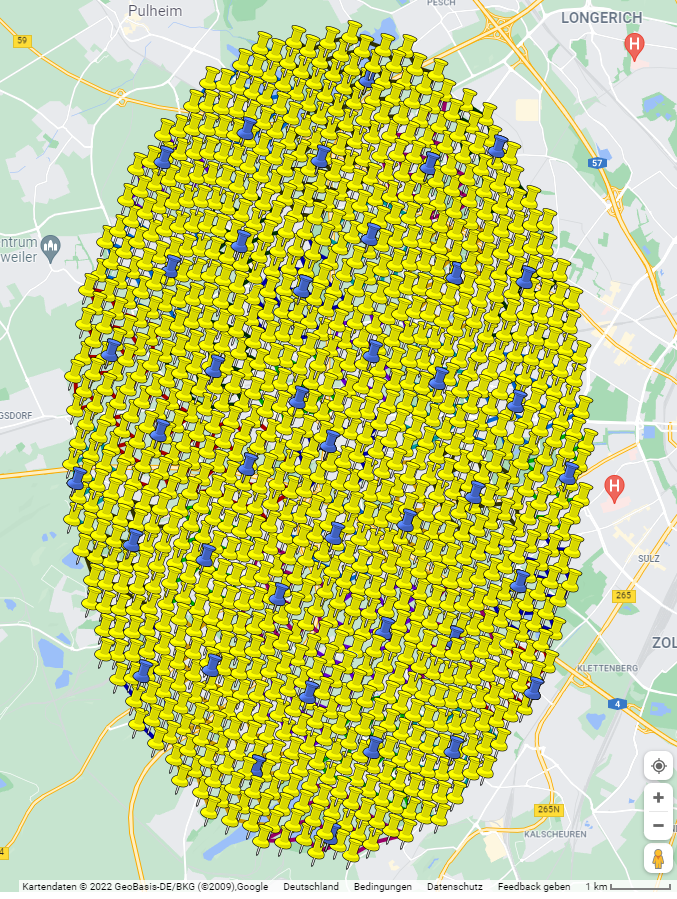
Figure: phyllotaxis, overview

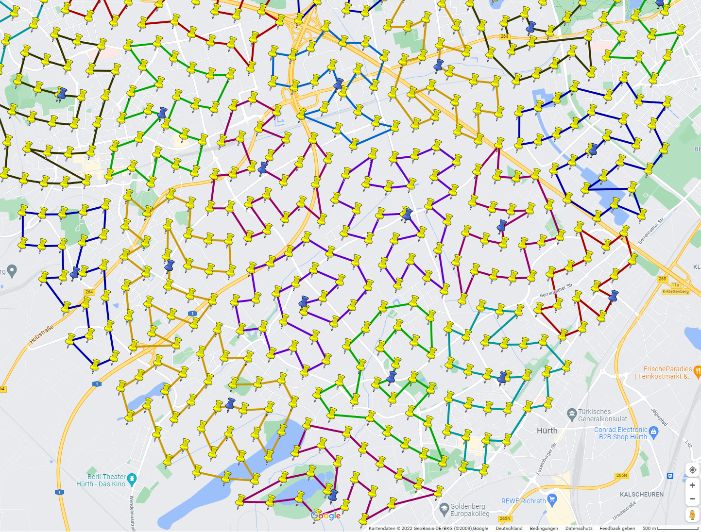
Figure: phyllotaxis, zoom

The zoomed view shows that the routes have approximately the same length, and that they neither cross each other nor have crossings within a route.

The example class ClusteringInnerCityExample.java builds phyllotaxis data of its own (1000 nodes and 50 resources) and is explained on the clustering example page. It has more elements than JOpt allows without a full license: License guide: element limits.

Phyllotaxis, example two

The second example modifies the first one: the nodes and resources are spread over two days. ClusteringInnerCityExample does this with the constant ADD_EVEN_ODD_SPLITTING set to true (the committed value is false): the nodes and resources with an even index, for example N_0 and R_0, are open or work on May 7, the others on May 6, each from 8 am to 10 pm (Europe/Berlin).

The clustering algorithm is expected to create clusters and routes that follow this changed setting as well (figure: phyllotaxis, odd and even).

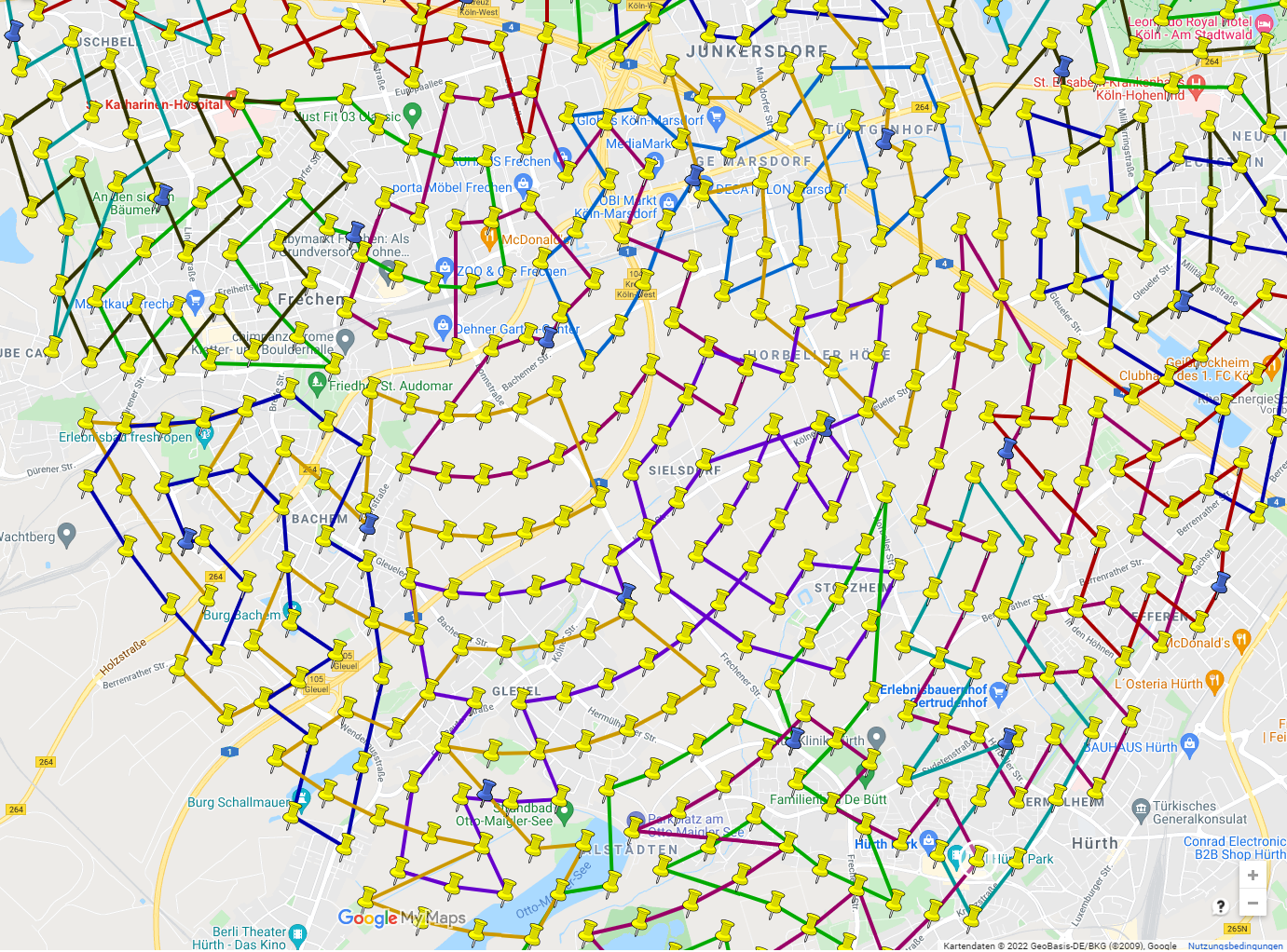
Figure: phyllotaxis, odd and even

From the combined figure alone, it is hard to see why it represents a good starting solution. The two figures below therefore show the odd and the even solution separately.

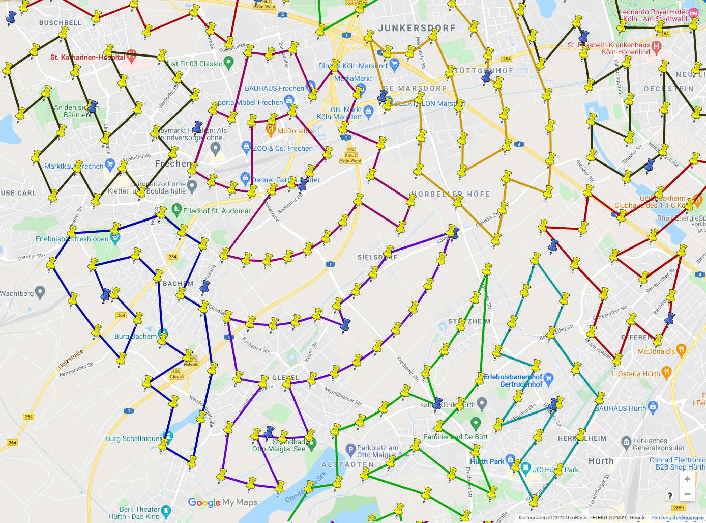
Figure: phyllotaxis, odd

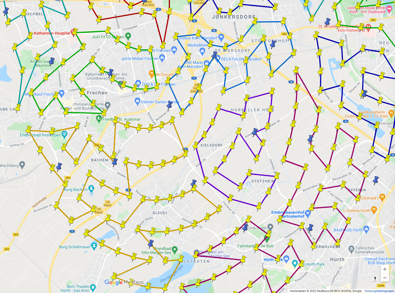
Figure: phyllotaxis, even

The clustering algorithm created two strictly separated sub-populations of clusters. Each solution in itself shows no crossings and routes of the same length.

City to city, example three

Besides inner-city multi-depot problems, the algorithm also needs to solve single-depot problems. This example is an effective single-depot problem covering Germany: the resources are positioned far away from each other, and the nodes are arranged in clusters (figure: Germany, overview).

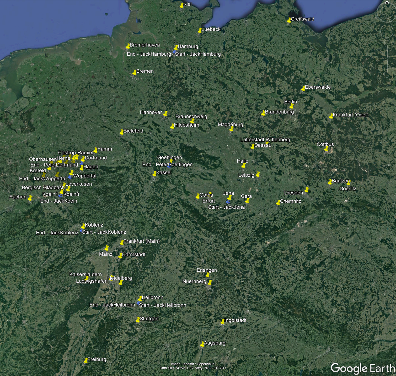
Figure: Germany, overview

The resources are expected to be used efficiently to reduce the overall distance. You can try to solve the problem by hand before you look at the constructed solution (figure: Germany, overview, solution).

Show the constructed solution

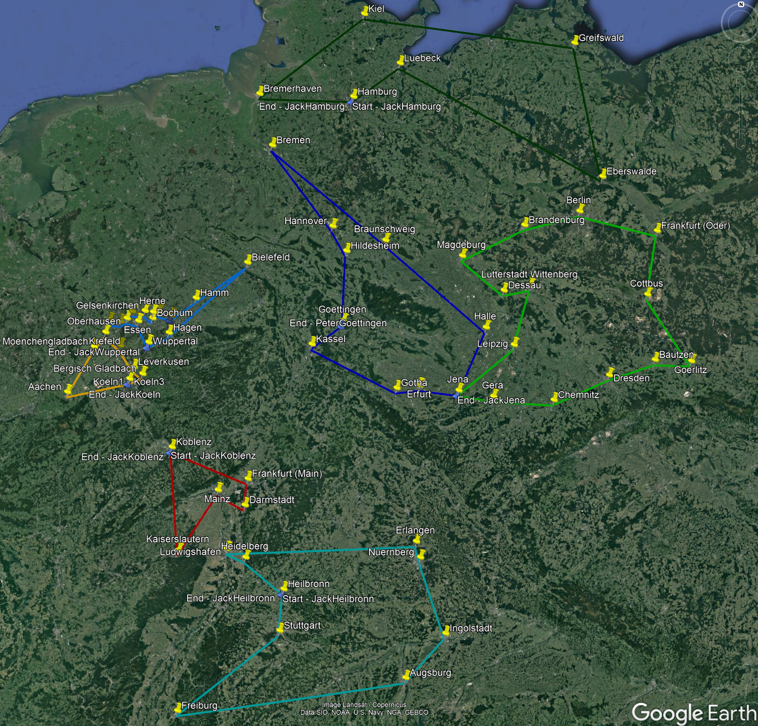
Figure: Germany, overview, solution

The north of the problem set shows the effect: the city of Eberswalde would usually be assigned to the light green route, which would cause overtime. The west, around the city of Essen, also shows a clear clustering.

When to use it

The construction runs by default at the start of an optimization. A run with the construction alone gives an approximate plan quickly, for example to show end customers before further optimization steps. To keep the clusters through the optimization, turn them into zones (see How to use it).

How to use it

To see the construction result alone, ClusteringInnerCityExample and ClusteringCityToCityExample set JOptExitCondition.JOptGenerationCount and JOpt.Algorithm.PreOptimization.SA.NumIterations to 0, so that no later optimization stage runs.

To keep the clusters during the optimization, the example ClusteringCityToCityKeepClustersForOptimizationExample sets JOpt.Clustering.AutoZoneCodeClusters and JOpt.Clustering.AutoZoneCodeClusters.isHard to True. The clusters found by the construction become zones, and as hard zones no node may leave its initial cluster during the optimization. ZoneCodes explains zones.

The expert example Algorithm selection shows how to choose the construction algorithm and the optimization phases.

In the JSON input of the REST service, the same keys go into optimizationOptions.properties as strings.

Properties

The clustering keys start with JOpt.Clustering.. Optimization properties lists them with their defaults, most of them under Construction properties, among them:

Limits

• With JOpt.Clustering.AutoZoneCodeClusters and JOpt.Clustering.AutoZoneCodeClusters.isHard set to true, no node may leave its initial cluster during the optimization.

Related examples

• Clustering example page: the three clustering examples explained, with their KML output
• ClusteringInnerCityExample.java: the construction on phyllotaxis data around a point in the west of Cologne (1000 nodes, 50 resources)
• ClusteringCityToCityExample.java: the construction on city-to-city data across Germany, with SmartConstructionAlgo
• ClusteringCityToCityKeepClustersForOptimizationExample.java: the clusters of this data kept as hard zones during the optimization

Related pages

• Introduction: how JOpt.TourOptimizer works: the construction, simulated annealing and genetic evolution in sequence
• Optimization properties: the property keys by category, with their defaults

Authors

DNA Evolutions GmbH

Added: 2026-01-03 (JOpt core 7.5.2-j17) | Last updated: 2026-10-23